This is part 2 in our series of posts on NBA lineups data. In the first post we added the lineups at each point of the game to the play-by-play table. Now, we are going to learn how to extract lineups plus minus and playing time from that table. In part 3, we will look at some stats from articles and show how to reproduce them. The output at the end of part 1 can be found here. After loading it, here’s what we have:
library(tidyverse)
library(lubridate)
library(zoo)
library(nbastatR)
library(future)

lineup_game <- read_csv("LineupGame0107.csv",
                        col_types = cols(timeQuarter = "c"))
## # A tibble: 461,344 x 25
## idGame numberEventMessageType numberEventActionT~ slugTeamHome slugTeamAway
## <dbl> <dbl> <dbl> <chr> <chr>
## 1 21900001 12 0 TOR NOP
## 2 21900001 10 0 TOR NOP
## 3 21900001 2 101 TOR NOP
## 4 21900001 4 0 TOR NOP
## 5 21900001 1 97 TOR NOP
## 6 21900001 2 6 TOR NOP
## 7 21900001 4 0 TOR NOP
## 8 21900001 2 75 TOR NOP
## 9 21900001 4 0 TOR NOP
## 10 21900001 2 103 TOR NOP
## # ... with 461,334 more rows, and 20 more variables: slugTeamPlayer1 <chr>,
## # slugTeamPlayer2 <chr>, slugTeamPlayer3 <chr>, numberPeriod <dbl>,
## # timeQuarter <chr>, secsPassedGame <dbl>, numberEvent <dbl>,
## # namePlayer1 <chr>, namePlayer2 <chr>, namePlayer3 <chr>,
## # descriptionPlayHome <chr>, descriptionPlayVisitor <chr>, ptsHome <dbl>,
## # ptsAway <dbl>, shotPtsHome <dbl>, shotPtsAway <dbl>,
## # marginBeforeHome <dbl>, marginBeforeAway <dbl>, lineupHome <chr>, ...There are 3 metrics we want to extract from this table: the number of points scored by a team and by its opponent during a lineup stint, and its duration. Thus, we need to know what the score and the time were at the beginning and at the end of a stint. In order to do this, we must understand how the NBA computes this type of data. Let’s look at a very common sequence in a NBA game: a player commits a foul, and the opponent goes to the line to shoot free throws. Between the first and second free throws, a team makes a substitution. Here’s an example from the first game of the season (Pelicans @ Raptors):
lineup_game %>%
  filter(idGame == 21900001,
         numberPeriod == 1,
         timeQuarter == "03:44") %>%
  select(starts_with("descriptionPlay"), starts_with("pts"))
## # A tibble: 4 x 4
## descriptionPlayHome descriptionPlayVisitor ptsHome ptsAway
## <chr> <chr> <dbl> <dbl>
## 1 <NA> Hart S.FOUL (P1.PN) (E.Dalen) 20 19
## 2 Siakam Free Throw 1 of 2 (7 PTS) <NA> 21 19
## 3 SUB: Gasol FOR Anunoby <NA> 21 19
## 4 Siakam Free Throw 2 of 2 (8 PTS) <NA> 22 19As you can see, at the moment the foul was called, the score was 20x19. Siakam makes the first free throw, making it 21x19, when Gasol replaced Anunoby. Should we say that Anunoby left the game when it was 21x19? The answer, surprisingly, is no. Since Anunoby was on the floor when the foul that led to the free throws was called, the NBA considers that every point that resulted from the free throws will count toward Anunoby when tracking his plus-minus. Therefore, we must find a way to account for that change when we calculate our metrics. A simple solution would be to just consider the score at the end of the second, since no time will go off the clock during the free throws:
lineup_game %>%
  filter(idGame == 21900001,
         numberPeriod == 1,
         timeQuarter == "03:44") %>%
  group_by(idGame, secsPassedGame) %>%
  mutate(ptsHome = ptsHome[row_number() == max(row_number())],
         ptsAway = ptsAway[row_number() == max(row_number())]) %>%
  ungroup() %>%
  select(starts_with("descriptionPlay"), starts_with("pts"))
## # A tibble: 4 x 4
## descriptionPlayHome descriptionPlayVisitor ptsHome ptsAway
## <chr> <chr> <dbl> <dbl>
## 1 <NA> Hart S.FOUL (P1.PN) (E.Dalen) 22 19
## 2 Siakam Free Throw 1 of 2 (7 PTS) <NA> 22 19
## 3 SUB: Gasol FOR Anunoby <NA> 22 19
## 4 Siakam Free Throw 2 of 2 (8 PTS) <NA> 22 19That would work for our example. But think about a different situation: at the end of the game, a team is shooting 2 free throws. Between the first and the second shot, there is a substitution, and the player makes the second free throw. However, before a full second has been taken off the clock, another foul is called. Now, the opposing team is shooting free throws, and there is another substitution in the middle of the shots. This is exactly what happened in a game early in the season between the Pistons and the Nets:
lineup_game %>%
  filter(idGame == 21900078,
         numberPeriod == 4,
         timeQuarter == "00:06") %>%
  select(starts_with("descriptionPlay"), starts_with("pts"))
## # A tibble: 11 x 4
## descriptionPlayHome descriptionPlayVisitor ptsHome ptsAway
## <chr> <chr> <dbl> <dbl>
## 1 <NA> Jordan Personal Take Foul (P~ 110 108
## 2 MISS Drummond Free Throw 1 of 2 <NA> 110 108
## 3 PISTONS Rebound <NA> 110 108
## 4 SUB: Morris FOR Kennard <NA> 110 108
## 5 Drummond Free Throw 2 of 2 (23~ <NA> 111 108
## 6 <NA> Nets Timeout: Regular (Reg.7~ 111 108
## 7 <NA> SUB: Temple FOR Jordan 111 108
## 8 Galloway Personal Take Foul (P~ <NA> 111 108
## 9 <NA> Prince Free Throw 1 of 2 (20~ 111 109
## 10 <NA> SUB: Jordan FOR Dinwiddie 111 109
## 11 <NA> MISS Prince Free Throw 2 of 2 111 109In this case, we can’t just replicate what we did earlier, because it would consider that Kennard left the game after the free throws attempted by Brooklyn, when the score was 111x109, when in fact he was supposed to leave with the score 111x108. To avoid this, we are going to create a column (canSub) to account for every substitution opportunity (fouls, dead ball turnovers, kickballs, team rebounds) and take the last value of each opportunity. Applying it to the previous case:
lineup_game %>%
  filter(idGame == 21900078,
         numberPeriod == 4,
         timeQuarter == "00:06") %>%
  mutate(canSub = case_when(numberEventMessageType == 5 & numberEventActionType %in% c(1, 2) ~ 1,     # dead ball turnovers
                            numberEventMessageType == 6 & numberEventActionType != 16 ~ 1,            # fouls
                            numberEventMessageType == 7 & numberEventActionType == 5 ~ 1,             # kickballs
                            numberEventMessageType == 4 & numberEventActionType == 0 & !str_detect(str_to_upper(descriptionPlayHome), "OFF:") ~ 1,
                            numberEventMessageType == 4 & numberEventActionType == 0 & !str_detect(str_to_upper(descriptionPlayVisitor), "OFF:") ~ 1,
                            TRUE ~ 0)) %>%
  group_by(idGame, secsPassedGame) %>%
  mutate(subOpp = cumsum(canSub)) %>%
  group_by(idGame, secsPassedGame, subOpp) %>%
  mutate(ptsHome = ptsHome[row_number() == max(row_number())],
         ptsAway = ptsAway[row_number() == max(row_number())]) %>%
  ungroup() %>%
  select(starts_with("descriptionPlay"), starts_with("pts"), subOpp)
## # A tibble: 11 x 5
## descriptionPlayHome descriptionPlayVisitor ptsHome ptsAway subOpp
## <chr> <chr> <dbl> <dbl> <dbl>
## 1 <NA> Jordan Personal Take Foul~ 111 108 1
## 2 MISS Drummond Free Throw 1~ <NA> 111 108 1
## 3 PISTONS Rebound <NA> 111 108 1
## 4 SUB: Morris FOR Kennard <NA> 111 108 1
## 5 Drummond Free Throw 2 of 2~ <NA> 111 108 1
## 6 <NA> Nets Timeout: Regular (Re~ 111 108 1
## 7 <NA> SUB: Temple FOR Jordan 111 108 1
## 8 Galloway Personal Take Fou~ <NA> 111 109 2
## 9 <NA> Prince Free Throw 1 of 2 ~ 111 109 2
## 10 <NA> SUB: Jordan FOR Dinwiddie 111 109 2
## 11 <NA> MISS Prince Free Throw 2 ~ 111 109 2Now Luke Kennard is leaving the game with the score at 111x108 and Dinwiddie is leaving the game with the score at 111x109, as we desired. There is, however, another case that needs to be accounted for. Take a look at this example, from the game between the Suns and the Raptors:
lineup_game %>%
  filter(idGame == 21900914,
         numberPeriod == 2,
         timeQuarter == "00:00") %>%
  select(numberEvent, starts_with("descriptionPlay"), starts_with("pts"))
## # A tibble: 8 x 5
## numberEvent descriptionPlayHome descriptionPlay~ ptsHome ptsAway
## <dbl> <chr> <chr> <dbl> <dbl>
## 1 234 Booker P.FOUL (P2.PN) (M.Lindsay) <NA> 68 59
## 2 235 <NA> MISS Boucher Fr~ 68 59
## 3 236 <NA> Raptors Rebound 68 59
## 4 237 SUB: Saric FOR Rubio <NA> 68 59
## 5 238 Booker T.FOUL (P2.PN) (M.Lindsay) <NA> 68 59
## 6 239 <NA> Lowry Free Thro~ 68 60
## 7 240 <NA> Boucher Free Th~ 68 61
## 8 241 <NA> <NA> 68 61There is a technical foul between free throws and just after a substitution. Is the potential point from a made technical free throw going to account for the player that goes in or the player that goes out? According to the NBA, the point from the technical foul shot by Lowry should go to Rubio, since the technical foul was called after he was subbed in the game. On the other hand, the point from the second free throw by Boucher, which was taken after the technical free throw, should go to Saric, since he was still in the game when the foul that generated the free throw happened. If it sounds confusing, it’s because it is. Our solution to this will be a little complicated as well. We’re going to reorder the events to make the free throw attempts from the same trip appear in sequence. In our current case, we need event number 240 to appear right after event 235. To do this, we’ll change the numberEvent of every second and third shot in a FT trip to the numberEvent of the first shot. Then, if there was a free throw in the sequence, we’ll take the last value of the sequence where the event was a free throw.
lineup_game %>%
  filter(idGame == 21900914) %>%
  mutate(canSub = case_when(numberEventMessageType == 5 & numberEventActionType %in% c(1, 2) ~ 1,     # dead ball turnovers
                            numberEventMessageType == 6 & numberEventActionType != 16 ~ 1,            # fouls
                            numberEventMessageType == 7 & numberEventActionType == 5 ~ 1,             # kickballs
                            numberEventMessageType == 4 & numberEventActionType == 0 & !str_detect(str_to_upper(descriptionPlayHome), "OFF:") ~ 1,
                            numberEventMessageType == 4 & numberEventActionType == 0 & !str_detect(str_to_upper(descriptionPlayVisitor), "OFF:") ~ 1,
                            TRUE ~ 0)) %>%
  group_by(idGame, secsPassedGame) %>%
  mutate(numberNew = ifelse(numberEventMessageType == 3 & numberEventActionType == 12,
                            paste(numberEvent[numberEventMessageType == 3 & numberEventActionType == 11], collapse = ", "),
                            as.character(numberEvent)),
         numberNew = ifelse(numberEventMessageType == 3 & numberEventActionType %in% c(14, 15),
                            paste(numberEvent[numberEventMessageType == 3 & numberEventActionType == 13], collapse = ", "),
                            numberNew)) %>%            # Note 1
  mutate(numberNew = str_split(numberNew, ", "),
         numberNew = map(numberNew, ~as.numeric(.)),
         numberNew = map2_dbl(numberNew, numberEvent, ~ max(.x[.x <= .y]))) %>%  # Note 2
  ungroup() %>%
  arrange(idGame, numberNew, numberEvent) %>%
  select(-numberNew) %>%
  group_by(idGame) %>%
  mutate(newptsHome = cumsum(shotPtsHome),
         newptsAway = cumsum(shotPtsAway)) %>%         # Note 3
  group_by(idGame, secsPassedGame) %>%
  mutate(subOpp = cumsum(canSub)) %>%
  group_by(idGame, secsPassedGame, subOpp) %>%
  mutate(hasFouls = sum(numberEventMessageType == 3)) %>%    # see if there is a foul in the sequence
  mutate(ptsHome = ifelse(hasFouls > 0,
                             newptsHome[row_number() == max(row_number()[numberEventMessageType == 3])],
                             newptsHome),     # take last value when the event is a free throw
         ptsAway = ifelse(hasFouls > 0,
                             newptsAway[row_number() == max(row_number()[numberEventMessageType == 3])],
                             newptsAway)) %>%
  ungroup() %>%
  filter(numberPeriod == 2,
         timeQuarter == "00:00") %>%
  select(numberEvent, starts_with("descriptionPlay"), starts_with("pts"))
## # A tibble: 8 x 5
## numberEvent descriptionPlayHome descriptionPlay~ ptsHome ptsAway
## <dbl> <chr> <chr> <dbl> <dbl>
## 1 234 Booker P.FOUL (P2.PN) (M.Lindsay) <NA> 68 60
## 2 235 <NA> MISS Boucher Fr~ 68 60
## 3 240 <NA> Boucher Free Th~ 68 60
## 4 236 <NA> Raptors Rebound 68 60
## 5 237 SUB: Saric FOR Rubio <NA> 68 60
## 6 238 Booker T.FOUL (P2.PN) (M.Lindsay) <NA> 68 61
## 7 239 <NA> Lowry Free Thro~ 68 61
## 8 241 <NA> <NA> 68 61- numberEventMessageType == 3 refers to FTs. The numberEventActionType descriptions are as follows:
- numberEventActionType == 11: free throw 1 of 2
- numberEventActionType == 12: free throw 2 of 2
- numberEventActionType == 13: free throw 1 of 3
- numberEventActionType == 14: free throw 2 of 3
- numberEventActionType == 15: free throw 3 of 3.
We are finding every first shot of a free throw trip inside a secsPassedGame.
- Then, we change the numberEvent of a second or third shot of a trip to be the maximum numberEvent between those first shots we found previously, as long as it was a numberEvent less than the one from the second or third shot (since the first free throw should happen before).
- We redo our score for each team with the new order where the free throws are put together.
Now we have Rubio leaving the game with the score already accounting for the second free throw, while the technical free throw is added to the lineup with Saric in the game. There’s just one more thing we must do: sometimes, a technical foul is called in between quarters. Then, at the start of the next quarter, a technical free throw is attempted, with the clock still at 12:00. Since there might be substitutions in between quarters, that free throw should count toward the lineup that starts the next quarter, according to the NBA. Therefore, we are going to do a little trick where we add a half second to our column secsPassedGame, which is what we use to group the events and adapt the points for the end of the lineups. Finally, here’s how our modified table will look like:
lineup_game_stats <- lineup_game %>%
  mutate(canSub = case_when(numberEventMessageType == 5 & !numberEventActionType %in% c(1, 2) ~ 1,    # dead ball turnovers
                            numberEventMessageType == 6 & numberEventActionType != 16 ~ 1,            # fouls
                            numberEventMessageType == 11 & numberEventActionType != 4 ~ 1,
                            numberEventMessageType == 7 & numberEventActionType == 5 ~ 1,             # kickballs
                            numberEventMessageType == 4 & numberEventActionType == 0 & !str_detect(str_to_upper(descriptionPlayHome), "OFF:") ~ 1,
                            numberEventMessageType == 4 & numberEventActionType == 0 & !str_detect(str_to_upper(descriptionPlayVisitor), "OFF:") ~ 1,
                            TRUE ~ 0)) %>%
  mutate(secsPassedGame2 = ifelse(timeQuarter == "12:00" &
                                    (str_detect(str_to_lower(descriptionPlayHome), "technical") |
                                       str_detect(str_to_lower(descriptionPlayVisitor), "technical")),
                                  secsPassedGame + 0.005, secsPassedGame)) %>%    # Note 4
  mutate(secsPassedGame2 = ifelse(timeQuarter == "00:00" & numberEventMessageType == 3 & numberEventActionType != 10,
                                  secsPassedGame2 - 0.1,
                                  secsPassedGame2)) %>%
  group_by(idGame, numberPeriod, secsPassedGame) %>%
  mutate(numberNew = ifelse(numberEventMessageType == 3 & numberEventActionType == 12,
                            paste(numberEvent[numberEventMessageType == 3 & numberEventActionType == 11], collapse = ", "),
                            as.character(numberEvent)),
         numberNew = ifelse(numberEventMessageType == 3 & numberEventActionType %in% c(14, 15),
                            paste(numberEvent[numberEventMessageType == 3 & numberEventActionType == 13], collapse = ", "),
                            numberNew)) %>%
  mutate(techs_and1 = sum(numberEventMessageType == 3 & numberEventActionType == 16) > 0 &
           sum(numberEventMessageType == 3 & numberEventActionType == 10) > 0 &
           sum(numberEventMessageType == 8) > 0) %>%
  mutate(numberNew = ifelse(numberEventMessageType == 3 & numberEventActionType == 10 & techs_and1,
                            paste(numberEvent[numberEventMessageType == 6 & numberEventActionType == 2 & techs_and1], collapse = ", "),
                            as.character(numberNew))) %>%
  mutate(numberNew = str_split(numberNew, ", "),
         numberNew = map(numberNew, ~as.numeric(.)),
         numberNew = map2_dbl(numberNew, numberEvent, ~ max(.x[.x <= .y]))) %>%
  ungroup() %>%
  arrange(idGame, numberNew, numberEvent) %>%
  group_by(idGame) %>%
  mutate(newptsHome = cumsum(shotPtsHome),
         newptsAway = cumsum(shotPtsAway)) %>%
  group_by(idGame, numberPeriod, secsPassedGame2) %>%
  mutate(subOpp = cumsum(canSub)) %>%
  group_by(idGame = as.character(idGame),
           numberPeriod = as.character(numberPeriod),
           subOpp,
           secsPassedGame2 = as.character(secsPassedGame2)) %>%
  mutate(hasFouls = sum(numberEventMessageType == 3)) %>%
  mutate(newptsHome = ifelse(hasFouls > 0,
                             newptsHome[row_number() == max(row_number()[numberEventMessageType == 3])],
                             newptsHome),
         newptsAway = ifelse(hasFouls > 0,
                             newptsAway[row_number() == max(row_number()[numberEventMessageType == 3])],
                             newptsAway)) %>%
  ungroup() %>%
  select(-c(secsPassedGame2, numberNew, techs_and1)) %>%
  mutate_all(~ as.character(.)) %>%
  mutate(secsPassedGame = as.numeric(secsPassedGame),
numberEvent = as.numeric(numberEvent))- If a technical free throw is taken with 12:00 in the clock, we add half a second to the secsPassedGame column, to differentiate from the secsPassedGame at 00:00 of the previous quarter.
Now our table looks like this:
lineup_game_stats## # A tibble: 461,344 x 30
## idGame numberEventMessageType numberEventActionT~ slugTeamHome slugTeamAway
## <chr> <chr> <chr> <chr> <chr>
## 1 21900001 12 0 TOR NOP
## 2 21900001 10 0 TOR NOP
## 3 21900001 2 101 TOR NOP
## 4 21900001 4 0 TOR NOP
## 5 21900001 1 97 TOR NOP
## 6 21900001 2 6 TOR NOP
## 7 21900001 4 0 TOR NOP
## 8 21900001 2 75 TOR NOP
## 9 21900001 4 0 TOR NOP
## 10 21900001 2 103 TOR NOP
## # ... with 461,334 more rows, and 25 more variables: slugTeamPlayer1 <chr>,
## # slugTeamPlayer2 <chr>, slugTeamPlayer3 <chr>, numberPeriod <chr>,
## # timeQuarter <chr>, secsPassedGame <dbl>, numberEvent <dbl>,
## # namePlayer1 <chr>, namePlayer2 <chr>, namePlayer3 <chr>,
## # descriptionPlayHome <chr>, descriptionPlayVisitor <chr>, ptsHome <chr>,
## # ptsAway <chr>, shotPtsHome <chr>, shotPtsAway <chr>,
## # marginBeforeHome <chr>, marginBeforeAway <chr>, lineupHome <chr>, ...We are now able to extract the lineups stats from it. As mentioned earlier, we want to get the initial and final score and time for each lineup stint. First, we are going to select only the columns we’ll need and turn our table into a long format (each line represents a team):
lineup_stats <- lineup_game_stats %>%
  select(idGame, numberEvent, slugTeamHome, slugTeamAway, numberPeriod, timeQuarter, secsPassedGame,
         newptsHome, newptsAway, lineupHome, lineupAway) %>%
  pivot_longer(cols = starts_with("lineup"),
               names_to = "lineupLocation",
               names_prefix = "lineup",
               values_to = "lineup") %>%
  mutate(ptsTeam = ifelse(lineupLocation == "Home", newptsHome, newptsAway),
         ptsOpp = ifelse(lineupLocation == "Away", newptsHome, newptsAway),
         slugTeam = ifelse(lineupLocation == "Home", slugTeamHome, slugTeamAway),
         slugOpp = ifelse(lineupLocation == "Away", slugTeamHome, slugTeamAway)) %>%
  distinct(idGame, slugTeam, slugOpp, numberPeriod, timeQuarter, secsPassedGame, ptsTeam, ptsOpp, lineup,
           teamLocation = lineupLocation, numberEvent) %>%
  arrange(idGame, numberEvent)

lineup_stats
## # A tibble: 922,688 x 11
## idGame numberEvent numberPeriod timeQuarter secsPassedGame lineup ptsTeam
## <chr> <dbl> <chr> <chr> <dbl> <chr> <chr>
## 1 21900001 1 1 12:00 0 Fred Va~ 0
## 2 21900001 1 1 12:00 0 Brandon~ 0
## 3 21900001 2 1 12:00 0 Fred Va~ 0
## 4 21900001 2 1 12:00 0 Brandon~ 0
## 5 21900001 3 1 11:48 12 Fred Va~ 0
## 6 21900001 3 1 11:48 12 Brandon~ 0
## 7 21900001 4 1 11:47 13 Fred Va~ 0
## 8 21900001 4 1 11:47 13 Brandon~ 0
## 9 21900001 5 1 11:47 13 Fred Va~ 0
## 10 21900001 5 1 11:47 13 Brandon~ 2
## # ... with 922,678 more rows, and 4 more variables: ptsOpp <chr>,
## # slugTeam <chr>, slugOpp <chr>, teamLocation <chr>Now we are going to identify every time there is a lineup change and create a column with the number of each stint. Then, we’ll get the initial and final score and time for them:
lineup_stats <- lineup_stats %>%
  group_by(idGame, slugTeam) %>%
  mutate(lineupChange = lineup != lag(lineup),
         lineupChange = coalesce(lineupChange, FALSE)) %>%
  group_by(idGame, slugTeam) %>%
  mutate(lineupStint = cumsum(lineupChange)) %>%
  ungroup() %>%
  arrange(idGame, lineupStint, numberEvent) %>%
  group_by(idGame, slugTeam, lineup, lineupStint) %>%
  summarise(initialScoreTeam = ptsTeam[row_number() == min(row_number())],
            initialScoreOpp = ptsOpp[row_number() == min(row_number())],
            finalScoreTeam = ptsTeam[row_number() == max(row_number())],
            finalScoreOpp =  ptsOpp[row_number() == max(row_number())],
            initialTime = secsPassedGame[row_number() == min(row_number())],
            finalTime = secsPassedGame[row_number() == max(row_number())]) %>%
  ungroup() %>%
  arrange(idGame, lineupStint) %>%
  group_by(idGame, slugTeam) %>%
  mutate(finalTime = ifelse(row_number() == max(row_number()), finalTime, lead(initialTime))) %>%
  ungroup()

lineup_stats
## # A tibble: 53,924 x 10
## idGame slugTeam lineup lineupStint initialScoreTeam initialScoreOpp
## <chr> <chr> <chr> <int> <chr> <chr>
## 1 21900001 NOP Brandon Ingra~ 0 0 0
## 2 21900001 TOR Fred VanVleet~ 0 0 0
## 3 21900001 NOP Brandon Ingra~ 1 19 18
## 4 21900001 TOR Fred VanVleet~ 1 12 17
## 5 21900001 NOP Brandon Ingra~ 2 19 18
## 6 21900001 TOR Fred VanVleet~ 2 16 19
## 7 21900001 NOP Brandon Ingra~ 3 19 18
## 8 21900001 TOR Fred VanVleet~ 3 22 19
## 9 21900001 NOP Brandon Ingra~ 4 19 20
## 10 21900001 TOR Kyle Lowry, M~ 4 25 22
## # ... with 53,914 more rows, and 4 more variables: finalScoreTeam <chr>,
## # finalScoreOpp <chr>, initialTime <dbl>, finalTime <dbl>Now we just need to calculate the net points and total time for each lineup in seconds:
lineup_stats <- lineup_stats %>%
mutate(across(c(contains("Score")), ~ as.numeric(.), .names = "{col}")) %>%
  mutate(totalScoreTeam = finalScoreTeam - initialScoreTeam,
         totalScoreOpp = finalScoreOpp - initialScoreOpp,
         netScoreTeam = totalScoreTeam - totalScoreOpp,
         totalTime = finalTime - initialTime) %>%
  arrange(idGame, lineupStint)
That’s it! We have the plus minus and the time played by each lineup stint in every game of the season! To make sure that everything worked fine, let’s compare the leaders in total plus minus from our table to the ones from NBA.com. First, we create a table with the individual stats for the players in each game:
indiv_stats <- lineup_stats %>%
  separate_rows(lineup, sep = ", ") %>%
  group_by(namePlayer = lineup, idGame, slugTeam) %>%
  summarise(totalPlusMinus = sum(netScoreTeam),
            totalSecs = sum(totalTime)) %>%
  ungroup() %>%
  arrange(-totalPlusMinus)

indiv_stats
## # A tibble: 20,501 x 5
## namePlayer idGame slugTeam totalPlusMinus totalSecs
## <chr> <chr> <chr> <dbl> <dbl>
## 1 James Harden 21900282 HOU 50 1841
## 2 Luka Doncic 21900208 DAL 45 1530
## 3 Giannis Antetokounmpo 21900882 MIL 44 1637
## 4 Caris LeVert 21900757 BKN 43 1602
## 5 Ja Morant 21900710 MEM 42 1651
## 6 Al Horford 21900928 PHI 41 2181
## 7 Dwight Powell 21900208 DAL 41 1486
## 8 Terance Mann 21900182 LAC 41 2000
## 9 Devin Booker 21900137 PHX 40 1944
## 10 Markelle Fultz 21900557 ORL 40 1852
## # ... with 20,491 more rowsNow let’s find the total plus minus and minutes for the season:
indiv_stats %>%
  group_by(namePlayer) %>%
  summarise(seasonPM = sum(totalPlusMinus),
            seasonSecs = sum(totalSecs)) %>%
  ungroup() %>%
  arrange(-seasonPM) %>%
  mutate(seasonMin = paste0(floor(seasonSecs / 60), ":", str_pad(round(seasonSecs %% 60, 0), side = "left", width = 2, pad = 0))) %>%
  select(-seasonSecs)
## # A tibble: 514 x 3
## namePlayer seasonPM seasonMin
## <chr> <dbl> <chr>
## 1 Giannis Antetokounmpo 648 1762:44
## 2 Khris Middleton 493 1653:11
## 3 LeBron James 483 2094:23
## 4 Brook Lopez 478 1622:25
## 5 Eric Bledsoe 456 1523:49
## 6 Jayson Tatum 440 2043:13
## 7 Wesley Matthews 425 1528:48
## 8 Donte DiVincenzo 409 1361:47
## 9 Kawhi Leonard 398 1643:07
## 10 Pascal Siakam 359 1882:30
## # ... with 504 more rows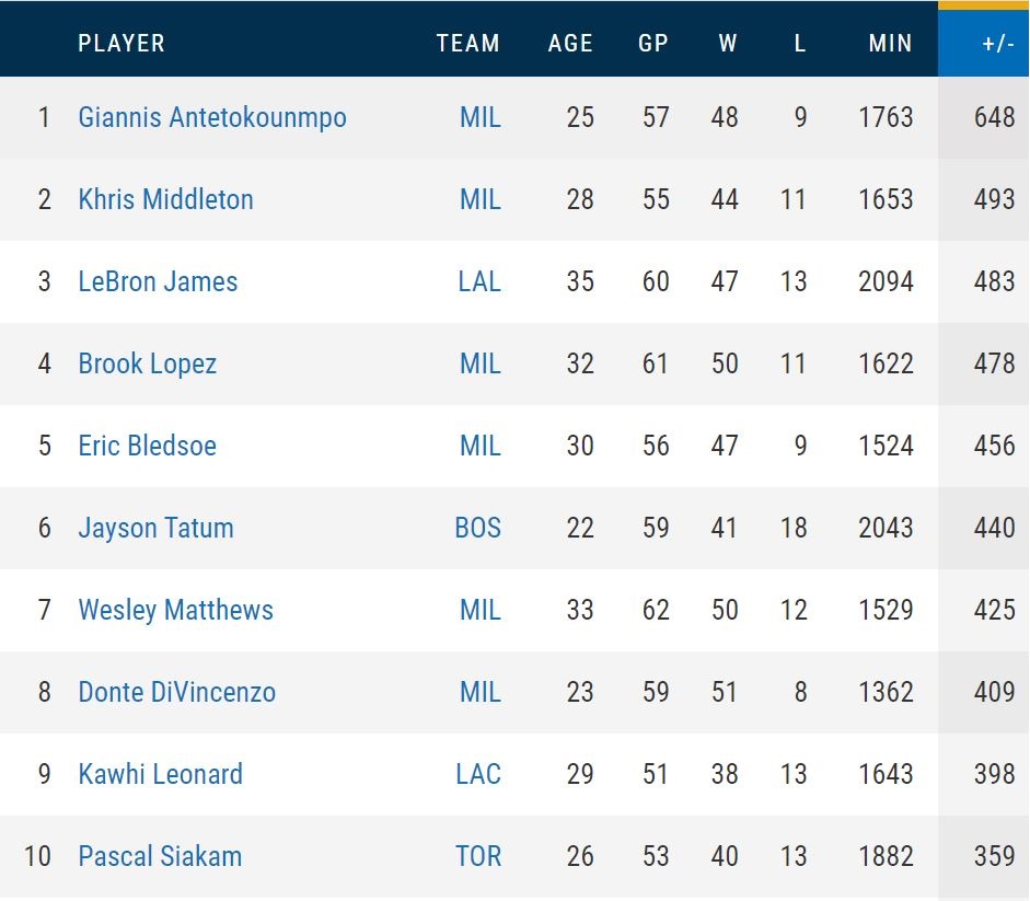
Now let’s compare find the top 10 lineups in total plus minus from our table to the one from NBA.com
lineup_stats %>%
  group_by(lineup) %>%
  summarise(seasonPM = sum(netScoreTeam),
            seasonSecs = sum(totalTime)) %>%
  ungroup() %>%
  arrange(-seasonPM) %>%
  mutate(seasonMin = paste0(floor(seasonSecs / 60), ":", str_pad(round(seasonSecs %% 60, 0), side = "left", width = 2, pad = 0))) %>%
  select(-seasonSecs)
## # A tibble: 17,150 x 3
## lineup seasonPM seasonMin
## <chr> <dbl> <chr>
## 1 Brook Lopez, Eric Bledsoe, Giannis Antetokounmpo, Khris M~ 180 407:47
## 2 Bojan Bogdanovic, Donovan Mitchell, Joe Ingles, Royce O'N~ 153 570:34
## 3 Gary Harris, Jamal Murray, Nikola Jokic, Paul Millsap, Wi~ 132 735:00
## 4 Brandon Ingram, Derrick Favors, Jrue Holiday, Lonzo Ball,~ 130 229:45
## 5 Chris Paul, Danilo Gallinari, Dennis Schroder, Shai Gilge~ 126 176:33
## 6 Bam Adebayo, Duncan Robinson, Jimmy Butler, Kendrick Nunn~ 121 487:42
## 7 Anthony Davis, Avery Bradley, Danny Green, JaVale McGee, ~ 98 389:19
## 8 Deandre Ayton, Devin Booker, Kelly Oubre Jr., Mikal Bridg~ 92 225:34
## 9 Bojan Bogdanovic, Donovan Mitchell, Mike Conley, Royce O'~ 75 380:46
## 10 Fred VanVleet, Kyle Lowry, Marc Gasol, OG Anunoby, Pascal~ 71 279:32
## # ... with 17,140 more rows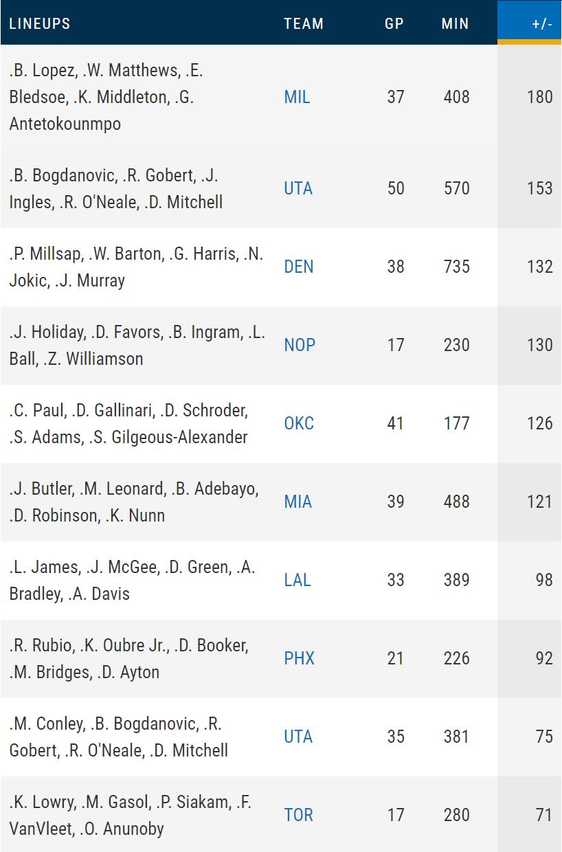
Everything seems to match. There are, however, very few discrepancies since there are some situations where even the NBA doesn’t know how to score the plus minus (e.g.: Danny Green shooting 2 free throws of a flagrant foul because Caldwell-Pope couldn’t stay in the game, but Green wasn’t supposed to be on the court when the foul was called in game 21900553. In the box score, Green’s +- is 9, but it’s 10 in the lineups page) and some due to game clock malfunctions (games 21900850 and 21900014). But those are very rare cases, so it’s safe to say that it won’t affect our results in e meaningful way. In our next post, we’re going to start reproducing some stats using our new data. Thank you for reading!