A few months ago, I created an account on Twitter to post code snippets reproducing some stats I saw in NBA-related posts and articles using the programming language R. All of the data came from the nbastatR package, and the stats I posted were often fairly simple to get to. However, I recently decided to try working with something a little more complicated: team lineups stats. It’s complicated because the R package doesn’t provide any lineup data, but it does provide play-by-play data. There, we can find all the substitutions and therefore arrive at the lineup that was on the court for each team at any given moment in the game. Then, we can analyze that data to answer questions about those lineups’ effectiveness on defense and offense, shooting and other metrics. This post will be the first in a series of posts showing how to get to that, then how to analyze it.
After installing the nbastatR and loading the required packages, the first step is to get all the games from the 2019-2020 season. We then filter out the preseason games and the All-Star weekend games (the current_schedule() function appears to not be currently working. However, you can find the output here)
library(tidyverse)
library(lubridate)
library(zoo)
library(nbastatR)   # devtools::install_github("abresler/nbastatR")
library(future)

team_logs <- game_logs(seasons = 2022, result_types = "team")

games <- team_logs %>%
  mutate(slugTeamHome = ifelse(locationGame == "H", slugTeam, slugOpponent),
         slugTeamAway = ifelse(locationGame == "A", slugTeam, slugOpponent)) %>%
  distinct(idGame, slugTeamHome, slugTeamAway)
We then get the play-by-play data for every game of the season:
plan(multiprocess)
play_logs_all <- play_by_play_v2(game_ids = unique(games$idGame))
The resulting output is a 461393 x 40 table:
play_logs_all## # A tibble: 461,393 x 40
## slugScore namePlayer1 teamNamePlayer1 slugTeamPlayer1 namePlayer2
## <chr> <chr> <chr> <chr> <chr>
## 1 <NA> <NA> <NA> <NA> <NA>
## 2 <NA> Marc Gasol Raptors TOR Derrick Favors
## 3 <NA> Lonzo Ball Pelicans NOP <NA>
## 4 <NA> Derrick Favors Pelicans NOP <NA>
## 5 2 - 0 Derrick Favors Pelicans NOP <NA>
## 6 <NA> OG Anunoby Raptors TOR <NA>
## 7 <NA> JJ Redick Pelicans NOP <NA>
## 8 <NA> Jrue Holiday Pelicans NOP <NA>
## 9 <NA> Fred VanVleet Raptors TOR <NA>
## 10 <NA> Kyle Lowry Raptors TOR <NA>
## # ... with 461,383 more rows, and 35 more variables: teamNamePlayer2 <chr>,
## # slugTeamPlayer2 <chr>, namePlayer3 <chr>, teamNamePlayer3 <chr>,
## # slugTeamPlayer3 <chr>, slugTeamLeading <chr>, idGame <dbl>,
## # numberEvent <dbl>, numberEventMessageType <dbl>,
## # numberEventActionType <dbl>, numberPeriod <dbl>, idPersonType1 <dbl>,
## # idPlayerNBA1 <dbl>, idTeamPlayer1 <dbl>, idPersonType2 <dbl>,
## # idPlayerNBA2 <dbl>, idTeamPlayer2 <dbl>, idPersonType3 <dbl>, ...We can see, however, that the data is not perfect. For example, there are some duplicate plays:
play_logs_all %>%
  select(idGame, numberEvent, numberPeriod, timeQuarter, descriptionPlayHome, descriptionPlayVisitor) %>%
  add_count(idGame, numberEvent, numberPeriod, timeQuarter, descriptionPlayHome, descriptionPlayVisitor) %>%
  filter(n > 1) %>%
  head(10)
## # A tibble: 10 x 7
## idGame numberEvent numberPeriod timeQuarter descriptionPlay~ descriptionPlay~
## <dbl> <dbl> <dbl> <chr> <chr> <chr>
## 1 2.19e7 527 4 10:10 MISS Markkanen ~ Ibaka BLOCK (2 ~
## 2 2.19e7 527 4 10:10 MISS Markkanen ~ Ibaka BLOCK (2 ~
## 3 2.19e7 215 2 6:50 Poole 29' 3PT P~ <NA>
## 4 2.19e7 215 2 6:50 Poole 29' 3PT P~ <NA>
## 5 2.19e7 198 2 7:48 Ross 26' 3PT Ju~ <NA>
## 6 2.19e7 198 2 7:48 Ross 26' 3PT Ju~ <NA>
## 7 2.19e7 324 2 1:53 <NA> MISS Randle 6' ~
## 8 2.19e7 324 2 1:53 <NA> MISS Randle 6' ~
## 9 2.19e7 341 3 10:41 MISS Brooks 11'~ Gobert BLOCK (3~
## 10 2.19e7 341 3 10:41 MISS Brooks 11'~ Gobert BLOCK (3~
## # ... with 1 more variable: n <int>And there are some event numbers that are out of order:
play_logs_all %>%
  select(idGame, numberEvent, numberPeriod, timeQuarter, descriptionPlayHome, descriptionPlayVisitor) %>%
  filter(idGame == 21900924,
         numberEvent > 75,
         numberEvent < 90)
## # A tibble: 12 x 6
## idGame numberEvent numberPeriod timeQuarter descriptionPlay~ descriptionPlay~
## <dbl> <dbl> <dbl> <chr> <chr> <chr>
## 1 2.19e7 86 1 6:29 SUB: Williams F~ <NA>
## 2 2.19e7 76 1 5:20 Lopez 2' Turnar~ <NA>
## 3 2.19e7 77 1 4:57 Williams BLOCK ~ MISS Sabonis 2'~
## 4 2.19e7 79 1 4:52 Williams REBOUN~ <NA>
## 5 2.19e7 80 1 4:50 MISS Middleton ~ <NA>
## 6 2.19e7 81 1 4:47 <NA> Warren REBOUND ~
## 7 2.19e7 82 1 4:43 <NA> MISS Warren 26'~
## 8 2.19e7 83 1 4:40 DiVincenzo REBO~ <NA>
## 9 2.19e7 84 1 4:30 Middleton 14' T~ <NA>
## 10 2.19e7 85 1 4:26 <NA> Pacers Timeout:~
## 11 2.19e7 88 1 4:26 SUB: Connaughto~ <NA>
## 12 2.19e7 89 1 4:26 <NA> SUB: Holiday FO~Consequently, we need to do some data cleaning. Besides the problems mentioned above, we are going to create our own scoring columns, the number of points scored in the play and the score margin before the play happened. That will help us in the future when analyzing clutch stats (score within 5 or less points with 5 or less minutes remaining in the 4th quarter or OT). We’ll also create a column to find the number of seconds passed in the game based on the quarter and the time remaining in it, to facilitate our work with time played by each player/lineup.
new_pbp <- play_logs_all %>%
  mutate(numberOriginal = numberEvent) %>%
  distinct(idGame, numberEvent, .keep_all = TRUE) %>%   # remove duplicate events
  mutate(secsLeftQuarter = (minuteRemainingQuarter * 60) + secondsRemainingQuarter) %>%
  mutate(secsStartQuarter = case_when(
    numberPeriod %in% c(1:5) ~ (numberPeriod - 1) * 720,
    TRUE ~ 2880 + (numberPeriod - 5) * 300
  )) %>%
  mutate(secsPassedQuarter = ifelse(numberPeriod %in% c(1:4), 720 - secsLeftQuarter, 300 - secsLeftQuarter),
         secsPassedGame = secsPassedQuarter + secsStartQuarter) %>%
  arrange(idGame, secsPassedGame) %>%
  filter(numberEventMessageType != 18) %>%     # instant replay
  group_by(idGame) %>%
  mutate(numberEvent = row_number()) %>%  # new numberEvent column with events in the right order
  ungroup() %>%
  select(idGame, numberOriginal, numberEventMessageType, numberEventActionType, namePlayer1, namePlayer2, namePlayer3,
         slugTeamPlayer1, slugTeamPlayer2,  slugTeamPlayer3, numberPeriod, timeQuarter, secsPassedGame,
         descriptionPlayHome, numberEvent, descriptionPlayVisitor) %>%
  mutate(shotPtsHome = case_when(
    numberEventMessageType == 3 & !str_detect(descriptionPlayHome, "MISS") ~ 1,
    numberEventMessageType == 1 & str_detect(descriptionPlayHome, "3PT") ~ 3,
    numberEventMessageType == 1 & !str_detect(descriptionPlayHome, "3PT") ~ 2,
    TRUE ~ 0
  )) %>%
  mutate(shotPtsAway = case_when(
    numberEventMessageType == 3 & !str_detect(descriptionPlayVisitor, "MISS") ~ 1,
    numberEventMessageType == 1 & str_detect(descriptionPlayVisitor, "3PT") ~ 3,
    numberEventMessageType == 1 & !str_detect(descriptionPlayVisitor, "3PT") ~ 2,
    TRUE ~ 0
  )) %>%
  group_by(idGame) %>%
  mutate(ptsHome = cumsum(shotPtsHome),
         ptsAway = cumsum(shotPtsAway)) %>%
  ungroup() %>%
  left_join(games) %>%
  select(idGame, numberOriginal, numberEventMessageType, numberEventActionType, slugTeamHome, slugTeamAway, slugTeamPlayer1,
         slugTeamPlayer2, slugTeamPlayer3, numberPeriod, timeQuarter, secsPassedGame, numberEvent, namePlayer1, namePlayer2,
         namePlayer3, descriptionPlayHome, descriptionPlayVisitor, ptsHome, ptsAway, shotPtsHome, shotPtsAway) %>%
  mutate(marginBeforeHome = ptsHome - ptsAway - shotPtsHome + shotPtsAway,
         marginBeforeAway = ptsAway - ptsHome - shotPtsAway + shotPtsHome,
timeQuarter = str_pad(timeQuarter, width = 5, pad = 0))- numberEventMessageType == 3 refers to FTs. We then filter out the ones where the FT was missed.
- numberEventMessageType == 1 refers to made FGs. We then find if the shot was a 3 or a 2 point FG.
- To find how many seconds have passed in a game, we first find how many seconds are left in each quarter.
- Then, we find how many seconds have passed at the start of each quarter. Here’s how the formula above works:
- when Period = 1 ~ (1 - 1) * 720 = 0 seconds of game time at the start of the quarter
- when Period = 2 ~ (2 - 1) * 720 = 720 seconds (12 minutes) of game time at the start of the quarter
- when Period = 3 ~ (3 - 1) * 720 = 1440 seconds (24 minutes) of game time at the start of the quarter
- when Period = 4 ~ (4 - 1) * 720 = 2160 seconds (36 minutes) of game time at the start of the quarter
- when Period = 5 (first OT) ~ (5 - 1) * 720 = 2880 seconds (48 minutes) of game time at the start of the quarter. After the 4th quarter, each OT adds only 300 seconds (5 minutes) to the game. Therefore:
- when Period = 6 (second OT) -> 2880 + (6 - 5) * 300 = 3180 seconds (53 minutes) of game time at the start of the quarter.
- Finally, we add the number of seconds of game time at the start of each quarter to the number of seconds of game time in each quarter (total seconds of each quarter - seconds left)
We now have a 459461 x 24 table with fewer columns but more complete with the information we are going to need. The next step will be to find the lineups for each team at every moment of the game. If we look at the play-by-play data, we can see that it shows every substitution that happened in the game, but it doesn’t show the lineups that start each quarter. In other words, if the team ends a quarter with a lineup but starts the next quarter with a different lineup, whatever substitution was made in between quarters will not appear in the play-by-play. Our first job then will be to find what lineups started each quarter. In order to find out if a player was on the floor at the beginning of a period, we must find if, in his first substitution, he was going in or out of the game. If he was going out, it means he was on the floor.
subs_made <- new_pbp %>%
  filter(numberEventMessageType == 8) %>%        # Note 6
  mutate(slugTeamLocation = ifelse(slugTeamPlayer1 == slugTeamHome, "Home", "Away")) %>%
  select(idGame, numberPeriod, timeQuarter, secsPassedGame, slugTeamPlayer = slugTeamPlayer1,
         slugTeamLocation, playerOut = namePlayer1, playerIn = namePlayer2) %>%
  pivot_longer(cols = starts_with("player"),
               names_to = "inOut",
               names_prefix = "player",
               values_to = "namePlayer") %>%
  group_by(idGame, numberPeriod, slugTeamPlayer, namePlayer) %>%
  filter(row_number() == 1) %>%
ungroup()- numberEventMessageType == 8 refers to substitutions.
However, it’s possible that a player played the entire quarter without being substituted. So let’s find every player who participated in an event in a quarter but none of those events was a substitution. We must also filter technical fouls out because a player can receive a technical while sitting on the bench.
others_qtr <- new_pbp %>%
  filter(numberEventMessageType != 8) %>%
  filter(!(numberEventMessageType == 6 & numberEventActionType %in% c(10, 11, 16, 18, 25))) %>%     # Note 7
  filter(!(numberEventMessageType == 11 & numberEventActionType %in% c(1, 4))) %>%   # Note 8
  pivot_longer(cols = starts_with("namePlayer"),
               names_to = "playerNumber",
               names_prefix = "namePlayer",
               values_to = "namePlayer") %>%
  mutate(slugTeamPlayer = case_when(playerNumber == 1 ~ slugTeamPlayer1,
                                    playerNumber == 2 ~ slugTeamPlayer2,
                                    playerNumber == 3 ~ slugTeamPlayer3,
                                    TRUE ~ "None")) %>%
  mutate(slugTeamLocation = ifelse(slugTeamPlayer == slugTeamHome, "Home", "Away")) %>%
  filter(!is.na(namePlayer),
         !is.na(slugTeamPlayer)) %>%
  anti_join(subs_made %>%
              select(idGame, numberPeriod, slugTeamPlayer, namePlayer)) %>%    # remove players that were subbed in the quarter
distinct(idGame, numberPeriod, namePlayer, slugTeamPlayer, slugTeamLocation)- numberEventMessageType == 6 & numberEventActionType %in% c(10, 11, 16, 18, 25) refer to technical fouls that can be called when a player is out of the game.
- numberEventMessageType == 11 & numberEventActionType == 1 refer to ejection due to second technical foul
Now we put together the players whose first substitution was going out and those who played the entire quarter. The output is the starting lineup in each quarter of every game for every team:
lineups_quarters <- subs_made %>%
  filter(inOut == "Out") %>%
  select(idGame, numberPeriod, slugTeamPlayer, namePlayer, slugTeamLocation) %>%
  bind_rows(others_qtr) %>%
  arrange(idGame, numberPeriod, slugTeamPlayer)

lineups_quarters
## # A tibble: 39,490 x 5
## idGame numberPeriod slugTeamPlayer namePlayer slugTeamLocation
## <dbl> <dbl> <chr> <chr> <chr>
## 1 21900001 1 NOP Lonzo Ball Away
## 2 21900001 1 NOP JJ Redick Away
## 3 21900001 1 NOP Derrick Favors Away
## 4 21900001 1 NOP Jrue Holiday Away
## 5 21900001 1 NOP Brandon Ingram Away
## 6 21900001 1 TOR Marc Gasol Home
## 7 21900001 1 TOR Kyle Lowry Home
## 8 21900001 1 TOR OG Anunoby Home
## 9 21900001 1 TOR Fred VanVleet Home
## 10 21900001 1 TOR Pascal Siakam Home
## # ... with 39,480 more rowsTo see if we got every lineup right, we need to see if there are 5 players in each period of each game:
lineups_quarters %>%
  count(idGame, numberPeriod, slugTeamPlayer) %>%
  filter(n != 5)
## # A tibble: 10 x 4
## idGame numberPeriod slugTeamPlayer n
## <dbl> <dbl> <chr> <int>
## 1 21900023 5 DEN 4
## 2 21900120 5 MIN 4
## 3 21900272 5 ATL 4
## 4 21900409 5 WAS 4
## 5 21900502 5 GSW 4
## 6 21900550 5 OKC 4
## 7 21900563 5 DET 4
## 8 21900696 5 SAC 4
## 9 21900787 5 ATL 4
## 10 21900892 5 HOU 4There are 10 occasions where we could only find 4 players who started in a quarter, all of them during OT, which is not surprising since there are fewer minutes and, consequently, fewer events to identify the players who took part in it. This happens when a player was on the court during all 5 minutes of OT but didn’t perform any action that appeared in the play-by-play. Here’s an example in the game 21900023 between Denver and Phoenix, from October 25th, 2019. This is the OT boxscore for Denver, from Basektball Reference:
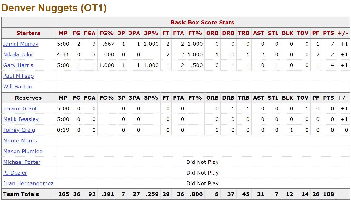
We can see that Malik Beasley played all 5 minutes of overtime but didn’t fill any box score column. The other 4 players who started for Denver in OT match the players we have in our output:
lineups_quarters %>%
  filter(idGame == 21900023,
         numberPeriod == 5,
         slugTeamPlayer == "DEN")
## # A tibble: 4 x 5
## idGame numberPeriod slugTeamPlayer namePlayer slugTeamLocation
## <dbl> <dbl> <chr> <chr> <chr>
## 1 21900023 5 DEN Nikola Jokic Home
## 2 21900023 5 DEN Jerami Grant Home
## 3 21900023 5 DEN Gary Harris Home
## 4 21900023 5 DEN Jamal Murray HomeUnfortunately, there’s nothing that can be done in this case to find out who the fifth player is when he doesn’t appear in the play-by-play data. Since there are only 10 such cases, we could look at the OT box scores from Basketball Reference and then add it manually. Here are the 10 players who are missing:
missing_players_ot <- tribble(
  ~idGame,   ~slugTeamPlayer,          ~namePlayer,     ~numberPeriod,
  21900023,        "DEN",           "Malik Beasley",          5,
  21900120,        "MIN",          "Treveon Graham",          5,
  21900272,        "ATL",         "De'Andre Hunter",          5,
  21900409,        "WAS",               "Ish Smith",          5,
  21900502,        "GSW",              "Damion Lee",          5,
  21900550,        "OKC",       "Terrance Ferguson",          5,
  21900563,        "DET",              "Tony Snell",          5,
  21900696,        "SAC",         "Harrison Barnes",          5,
  21900787,        "ATL",         "De'Andre Hunter",          5,
  21900892,        "HOU",             "Eric Gordon",          5,
  21901281,        "DEN",            "Monte Morris",          6
) %>%
  left_join(games) %>%
  mutate(slugTeamLocation = ifelse(slugTeamHome == slugTeamPlayer, "Home", "Away")) %>%
  select(-c(slugTeamHome, slugTeamAway))
Binding it to the original table:
lineups_quarters <- lineups_quarters %>%
  bind_rows(missing_players_ot) %>%
  arrange(idGame, numberPeriod, slugTeamPlayer)
Now we are going to work with the substitutions from our clean play-by-play data. Whenever there is a sub (numberEventMessageType == 8), namePlayer1 represents the player coming out and namePlayer2 represents the player going in. We want to have a column that tells us what the lineup was before the substitution and the resulting lineup after. In order to do that, we need a base value to use as the lineup before the first substitution, and that will be exactly the starting lineups for each quarter we just got. So we join the first substitution with the starting lineup, which will now be called lineupBefore.
lineup_subs <- new_pbp %>%
  filter(numberEventMessageType == 8) %>%
  select(idGame, numberPeriod, timeQuarter, secsPassedGame, slugTeamPlayer = slugTeamPlayer1, playerOut = namePlayer1,
         playerIn = namePlayer2, numberEvent) %>%
  arrange(idGame, numberEvent) %>%
  group_by(idGame, numberPeriod, slugTeamPlayer) %>%
  mutate(row1 = row_number()) %>%
  ungroup() %>%
  left_join(lineups_quarters %>%
              group_by(idGame, numberPeriod, slugTeamPlayer) %>%
              summarise(lineupBefore = paste(sort(unique(namePlayer)), collapse = ", ")) %>%
              ungroup() %>%
              mutate(row1 = 1)) %>%
  select(-row1)

lineup_subs
## # A tibble: 47,614 x 9
## idGame numberPeriod timeQuarter secsPassedGame slugTeamPlayer playerOut
## <dbl> <dbl> <chr> <dbl> <chr> <chr>
## 1 21900001 1 06:36 324 TOR Marc Gasol
## 2 21900001 1 05:20 400 TOR Kyle Lowry
## 3 21900001 1 04:46 434 NOP Lonzo Ball
## 4 21900001 1 04:46 434 NOP JJ Redick
## 5 21900001 1 04:46 434 NOP Derrick Favo~
## 6 21900001 1 04:16 464 NOP Jrue Holiday
## 7 21900001 1 04:16 464 NOP Brandon Ingr~
## 8 21900001 1 03:44 496 TOR OG Anunoby
## 9 21900001 1 02:44 556 TOR Fred VanVleet
## 10 21900001 1 01:26 634 TOR Pascal Siakam
## # ... with 47,604 more rows, and 3 more variables: playerIn <chr>,
## # numberEvent <int>, lineupBefore <chr>The next step is a little complicated. We are going to replace the player coming out with the player going in from our lineupBefore column. Then, after each sub, our new lineupBefore will be the previous resulting lineup (lineupAfter).
lineup_subs <- lineup_subs %>%
  mutate(lineupBefore = str_split(lineupBefore, ", ")) %>%
  arrange(idGame, numberEvent) %>%
  group_by(idGame, numberPeriod, slugTeamPlayer) %>%
  mutate(lineupAfter = accumulate2(playerIn, playerOut, ~setdiff(c(..1, ..2), ..3), .init = lineupBefore[[1]])[-1],
         lineupBefore = coalesce(lineupBefore, lag(lineupAfter))) %>%
  ungroup() %>%
  mutate_all(~map_chr(., ~paste(.x, collapse = ", "))) %>%
  mutate_at(vars("numberEvent", "numberPeriod", "idGame"), ~ as.integer(.)) %>%
  mutate(secsPassedGame = as.numeric(secsPassedGame)) %>%
  arrange(idGame, numberEvent) %>%
  left_join(lineups_quarters %>%
              distinct(idGame, slugTeamPlayer, slugTeamLocation)) %>%
  filter(!is.na(slugTeamLocation))

lineup_subs %>%
  select(lineupBefore, playerOut, playerIn, lineupAfter) %>%
  head(10)
## # A tibble: 10 x 4
## lineupBefore playerOut playerIn lineupAfter
## <chr> <chr> <chr> <chr>
## 1 Fred VanVleet, Kyle Lowry,~ Marc Gasol Serge Ibaka Fred VanVleet, Kyle Lowr~
## 2 Fred VanVleet, Kyle Lowry,~ Kyle Lowry Norman Pow~ Fred VanVleet, OG Anunob~
## 3 Brandon Ingram, Derrick Fa~ Lonzo Ball Josh Hart Brandon Ingram, Derrick ~
## 4 Brandon Ingram, Derrick Fa~ JJ Redick Jahlil Oka~ Brandon Ingram, Derrick ~
## 5 Brandon Ingram, Derrick Fa~ Derrick Fa~ E'Twaun Mo~ Brandon Ingram, Jrue Hol~
## 6 Brandon Ingram, Jrue Holid~ Jrue Holid~ Nickeil Al~ Brandon Ingram, Josh Har~
## 7 Brandon Ingram, Josh Hart,~ Brandon In~ Kenrich Wi~ Josh Hart, Jahlil Okafor~
## 8 Fred VanVleet, OG Anunoby,~ OG Anunoby Marc Gasol Fred VanVleet, Pascal Si~
## 9 Fred VanVleet, Pascal Siak~ Fred VanVl~ Kyle Lowry Pascal Siakam, Serge Iba~
## 10 Pascal Siakam, Serge Ibaka~ Pascal Sia~ OG Anunoby Serge Ibaka, Norman Powe~We now have all the substitutions we need, with the lineups before and after they took place. We just need to add it to the play-by-play data, first by joining the starting lineup and then the lineups after each substitution. We do want to have both the home team and the away team lineups at every point in the game, in order to later analyze different match-ups. Therefore, we need to widen our table to separate it between team locations before joining in.
lineup_game <- new_pbp %>%
  group_by(idGame, numberPeriod) %>%
  mutate(row1 = row_number()) %>%
  ungroup() %>%
  left_join(lineups_quarters %>%
              group_by(idGame, numberPeriod, slugTeamLocation) %>%
              summarise(lineupBefore = paste(sort(unique(namePlayer)), collapse = ", ")) %>%
              ungroup() %>%
              pivot_wider(names_from = slugTeamLocation,
                          names_prefix = "lineupInitial",
                          values_from = lineupBefore) %>%
              mutate(row1 = 1)) %>%
  select(-row1) %>%
  left_join(lineup_subs %>%
              mutate(lineupBeforeHome = ifelse(slugTeamLocation == "Home", lineupBefore, NA),
                     lineupAfterHome = ifelse(slugTeamLocation == "Home", lineupAfter, NA),
                     lineupBeforeAway = ifelse(slugTeamLocation == "Away", lineupBefore, NA),
                     lineupAfterAway = ifelse(slugTeamLocation == "Away", lineupAfter, NA)) %>%
              select(idGame, numberPeriod, timeQuarter, secsPassedGame, numberEvent, slugTeamPlayer1 = slugTeamPlayer,
                     contains("Home"), contains("Away"))) %>%
  mutate_at(vars(c(lineupBeforeHome, lineupAfterHome)), ~ ifelse(!is.na(lineupInitialHome), lineupInitialHome, .)) %>%
  mutate_at(vars(c(lineupBeforeAway, lineupAfterAway)), ~ ifelse(!is.na(lineupInitialAway), lineupInitialAway, .)) %>%
  select(-starts_with("lineupInitial"))
We have the lineups before and after every substitution, but we also need the lineups for every other event. Thus, the lineups in every event between subs will be lineup after the last sub.
lineup_game <- lineup_game %>%
  group_by(idGame, numberPeriod) %>%
  mutate(lineupHome = na.locf(lineupAfterHome, na.rm = FALSE),
         lineupAway = na.locf(lineupAfterAway, na.rm = FALSE),
         lineupHome = ifelse(is.na(lineupHome), na.locf(lineupBeforeHome, fromLast = TRUE, na.rm = FALSE), lineupHome),
         lineupAway = ifelse(is.na(lineupAway), na.locf(lineupBeforeAway, fromLast = TRUE, na.rm = FALSE), lineupAway),
         lineupHome = str_split(lineupHome, ", "),
         lineupAway = str_split(lineupAway, ", "),
         lineupHome = map_chr(lineupHome, ~ paste(sort(.), collapse = ", ")),
         lineupAway = map_chr(lineupAway, ~ paste(sort(.), collapse = ", "))) %>%
  ungroup() %>%
  select(-c(starts_with("lineupBefore"), starts_with("lineupAfter")))

lineup_game
## # A tibble: 459,461 x 26
## idGame numberOriginal numberEventMessageType numberEventActio~ slugTeamHome
## <dbl> <dbl> <dbl> <dbl> <chr>
## 1 21900001 2 12 0 TOR
## 2 21900001 4 10 0 TOR
## 3 21900001 7 2 101 TOR
## 4 21900001 8 4 0 TOR
## 5 21900001 9 1 97 TOR
## 6 21900001 10 2 6 TOR
## 7 21900001 11 4 0 TOR
## 8 21900001 12 2 75 TOR
## 9 21900001 13 4 0 TOR
## 10 21900001 14 2 103 TOR
## # ... with 459,451 more rows, and 21 more variables: slugTeamAway <chr>,
## # slugTeamPlayer1 <chr>, slugTeamPlayer2 <chr>, slugTeamPlayer3 <chr>,
## # numberPeriod <dbl>, timeQuarter <chr>, secsPassedGame <dbl>,
## # numberEvent <int>, namePlayer1 <chr>, namePlayer2 <chr>, namePlayer3 <chr>,
## # descriptionPlayHome <chr>, descriptionPlayVisitor <chr>, ptsHome <dbl>,
## # ptsAway <dbl>, shotPtsHome <dbl>, shotPtsAway <dbl>,
## # marginBeforeHome <dbl>, marginBeforeAway <dbl>, lineupHome <chr>, ...There it is! We have the lineups for the home and away team for every play in the play-by-play data. In the next post, I’ll show how to analyze some stats using it. Thanks for reading!