This is part 4 in our series of posts on NBA lineups data. In the last post we learned how to find the performance of different combinations of lineups. Now, we are going to reproduce some other stats when different players are on or off the court. In this post, the tables used will be the play-by-play with lineups added, and the lineups stats. We are also going to get every shot taken in the regular season until now. Here’s how to do it:
library(nbastatR)
library(future)

game_logs <- game_logs(seasons = 2020)

games <- game_logs %>%
  select(idGame, slugTeam, slugOpponent, locationGame) %>%
  mutate(slugTeamHome = ifelse(locationGame == "H", slugTeam, slugOpponent),
         slugTeamAway = ifelse(locationGame == "A", slugTeam, slugOpponent)) %>%
  select(-c(slugTeam, slugOpponent, locationGame)) %>%
  distinct(idGame, .keep_all = TRUE)

plan(multiprocess)
shots_2020 <- teams_shots(teams = unique(games$nameTeamAway),
                          seasons = 2020)
The final output can be found here. Let’s load our other tables:
library(tidyverse)

lineup_game <- read_csv("LineupGame0107.csv",
                        col_types = cols(timeQuarter = "c"))

lineup_stats <- read_csv("https://raw.githubusercontent.com/ramirobentes/NBAblog/master/LineupStatsNBA.csv")
All the numbers in the post come from John Schuhmann’s Film Study columns. First, let’s find the players with the highest assist percentage while on the floor:

Here’s the thought process: we’are going to filter our table and keep only the rows where there was a made field goal (numberEventMessageType = 1). In these rows, the namePlayer1 column always refers to the player who made the field goal, while namePlayer2 refers to the one who had the assist. To calculate assist percentage, we need to find the number of total assists by a player and divide it by the number of field goals while he was on the floor but wasn’t the shooter. With that in mind, we create a column with every player who was not involved in the play (not_involved), which will be the difference between the lineup that was on the floor the namePlayers 1 and 2.
assist_pct_players <- lineup_game %>%
  filter(numberEventMessageType == 1) %>%
  mutate(lineup = ifelse(slugTeamPlayer1 == slugTeamHome, lineupHome, lineupAway)) %>%
  select(idGame, numberEvent, slugTeamPlayer1, scorer = namePlayer1, assist = namePlayer2, lineup) %>%
  mutate(lineup = str_split(lineup, ", ")) %>%
  mutate(not_involved = map2(assist, lineup, ~ setdiff(.y, .x)),
         not_involved = map2(scorer, not_involved, ~ setdiff(.y, .x)),
         not_involved = map_chr(not_involved, ~ paste(sort(.), collapse = ", ")))

assist_pct_players
## # A tibble: 79,292 x 7
## idGame numberEvent slugTeamPlayer1 scorer assist lineup not_involved
## <dbl> <dbl> <chr> <chr> <chr> <list> <chr>
## 1 21900001 5 NOP Derric~ <NA> <chr [~ Brandon Ingram,~
## 2 21900001 18 NOP Brando~ <NA> <chr [~ Derrick Favors,~
## 3 21900001 20 TOR OG Anu~ Fred V~ <chr [~ Kyle Lowry, Mar~
## 4 21900001 21 NOP Lonzo ~ Brando~ <chr [~ Derrick Favors,~
## 5 21900001 27 NOP Brando~ Jrue H~ <chr [~ Derrick Favors,~
## 6 21900001 33 NOP JJ Red~ Lonzo ~ <chr [~ Brandon Ingram,~
## 7 21900001 36 NOP JJ Red~ Jrue H~ <chr [~ Brandon Ingram,~
## 8 21900001 37 TOR Pascal~ <NA> <chr [~ Fred VanVleet, ~
## 9 21900001 41 NOP Derric~ Lonzo ~ <chr [~ Brandon Ingram,~
## 10 21900001 42 TOR Fred V~ Pascal~ <chr [~ Kyle Lowry, Mar~
## # ... with 79,282 more rowsNow that we have the players who scored, who had the assist and who were not involved, we’ll turn the rows into each player’s “participation” in the play and then count them:
assist_pct_players <- assist_pct_players %>%
  separate_rows(not_involved, sep = ", ") %>%
  pivot_longer(cols = c("scorer", "assist", "not_involved"),
               names_to = "participation",
               values_to = "namePlayer") %>%
  distinct(idGame, numberEvent, slugTeamPlayer1, participation, namePlayer) %>%
  count(namePlayer, participation)

assist_pct_players
## # A tibble: 1,501 x 3
## namePlayer participation n
## <chr> <chr> <int>
## 1 Aaron Gordon assist 215
## 2 Aaron Gordon not_involved 1098
## 3 Aaron Gordon scorer 314
## 4 Aaron Holiday assist 193
## 5 Aaron Holiday not_involved 817
## 6 Aaron Holiday scorer 202
## 7 Abdel Nader assist 35
## 8 Abdel Nader not_involved 466
## 9 Abdel Nader scorer 100
## 10 Adam Mokoka assist 4
## # ... with 1,491 more rowsNow we can calculate the assist percentage, and filter by the number of game and minutes per game using our lineup_stats table:
assist_pct_players %>%
  pivot_wider(names_from = participation,
              values_from = n) %>%
  mutate(pct_assist = assist / (assist + not_involved)) %>%
  arrange(-pct_assist) %>%
  left_join(lineup_stats %>%
              separate_rows(lineup, sep = ", ") %>%
              group_by(namePlayer = lineup) %>%
              summarise(totalTime = sum(totalTime),
                        games = n_distinct(idGame)) %>%
              ungroup()) %>%
  filter(games >= 25,
         round((totalTime / games / 60), 1) >= 20) %>%
  select(-c(totalTime, games))
## # A tibble: 226 x 5
## namePlayer assist not_involved scorer pct_assist
## <chr> <int> <int> <int> <dbl>
## 1 LeBron James 636 687 586 0.481
## 2 Luka Doncic 470 578 512 0.448
## 3 Trae Young 560 763 546 0.423
## 4 Ricky Rubio 507 835 252 0.378
## 5 Derrick Rose 278 467 369 0.373
## 6 James Harden 450 815 603 0.356
## 7 Malcolm Brogdon 343 629 289 0.353
## 8 Ja Morant 409 767 393 0.348
## 9 Elfrid Payton 323 607 193 0.347
## 10 Devonte' Graham 471 896 368 0.345
## # ... with 216 more rowsEverything matches with the number from the article!
Our second stat will be the rebounding percentage of every lineup that has played at least 150 minutes together:

Here, we’re going to filter our table and keep only the rows where there was a rebound (numberEventMessageType = 4 and numberEventActionType = 0). Then, we want the rows to correspond to the rebound opportunity for each team. In other words, for every rebound, we want to know the lineup that got it and the one that gave it up:
rebound_pct_lineups <- lineup_game %>%
  filter(numberEventMessageType == 4 & numberEventActionType == 0) %>%
  pivot_longer(cols = starts_with("lineup"),
               names_to = "lineupLocation",
               names_prefix = "lineup",
               values_to = "lineup") %>%
  select(idGame, numberEvent, slugTeamHome, slugTeamAway, descriptionPlayHome, descriptionPlayVisitor, lineup, lineupLocation)

rebound_pct_lineups
## # A tibble: 196,594 x 8
## idGame numberEvent slugTeamHome slugTeamAway descriptionPlayHome
## <dbl> <dbl> <chr> <chr> <chr>
## 1 21900001 4 TOR NOP <NA>
## 2 21900001 4 TOR NOP <NA>
## 3 21900001 7 TOR NOP <NA>
## 4 21900001 7 TOR NOP <NA>
## 5 21900001 9 TOR NOP VanVleet REBOUND (Off:0 Def:1)
## 6 21900001 9 TOR NOP VanVleet REBOUND (Off:0 Def:1)
## 7 21900001 11 TOR NOP <NA>
## 8 21900001 11 TOR NOP <NA>
## 9 21900001 13 TOR NOP Lowry REBOUND (Off:0 Def:1)
## 10 21900001 13 TOR NOP Lowry REBOUND (Off:0 Def:1)
## # ... with 196,584 more rows, and 3 more variables:
## # descriptionPlayVisitor <chr>, lineup <chr>, lineupLocation <chr>Now we need to create a column to tell us whether the team got the rebound or if its opponent did. Then, we count the number of times each situation occurred for every lineup, and calculate the rebound percentage (number of rebounds a team got divided by the total available rebounds). Finally, we filter to keep only the lineups that have played at least 150 minutes together:
rebound_pct_lineups %>%
  mutate(gotReb = case_when(!is.na(descriptionPlayHome) & lineupLocation == "Home" ~ "team",
                            !is.na(descriptionPlayVisitor) & lineupLocation == "Away" ~ "team",
                            TRUE ~ "opponent")) %>%
  count(lineup, gotReb) %>%
  pivot_wider(names_from = gotReb,
              values_from = n) %>%
  mutate(pct_rebound = team / (team + opponent)) %>%
  arrange(pct_rebound) %>%
  left_join(lineup_stats %>%
              group_by(lineup) %>%
              summarise(totalTime = sum(totalTime)) %>%
              ungroup() %>%
              select(lineup, totalTime)) %>%
  filter(totalTime >= 9000) %>%
  select(lineup, team, opponent, pct_rebound)
## # A tibble: 50 x 4
## lineup team opponent pct_rebound
## <chr> <int> <int> <dbl>
## 1 Al Horford, Ben Simmons, Furkan Korkmaz, Matisse ~ 132 169 0.439
## 2 Fred VanVleet, Marc Gasol, Norman Powell, OG Anun~ 179 210 0.460
## 3 Bradley Beal, Isaiah Thomas, Rui Hachimura, Thoma~ 175 205 0.461
## 4 Danuel House Jr., James Harden, P.J. Tucker, Robe~ 166 191 0.465
## 5 Aaron Holiday, Domantas Sabonis, Doug McDermott, ~ 234 263 0.471
## 6 Bojan Bogdanovic, Donovan Mitchell, Joe Ingles, M~ 223 246 0.475
## 7 Daniel Theis, Gordon Hayward, Jaylen Brown, Jayso~ 171 185 0.480
## 8 Fred VanVleet, Kyle Lowry, OG Anunoby, Pascal Sia~ 195 210 0.481
## 9 Chris Paul, Danilo Gallinari, Luguentz Dort, Shai~ 148 159 0.482
## 10 Buddy Hield, De'Aaron Fox, Harrison Barnes, Neman~ 175 188 0.482
## # ... with 40 more rowsThere are some decimal point discrepancies with the values from the article and NBA.com. That’s due to some events in the play-by-play data being out of order (e.g.: substitution appears after a rebound from a missed free throw).
lineup_game %>%
  filter(idGame == 21900466,
         secsPassedGame == 158) %>%
  select(descriptionPlayHome, descriptionPlayVisitor)
## # A tibble: 5 x 2
## descriptionPlayHome descriptionPlayVisitor
## <chr> <chr>
## 1 Tatum S.FOUL (P1.T2) (R.Acosta) <NA>
## 2 <NA> Love Free Throw 1 of 2 (3 PTS)
## 3 <NA> MISS Love Free Throw 2 of 2
## 4 Hayward REBOUND (Off:0 Def:1) <NA>
## 5 SUB: Kanter FOR Theis <NA>For our next two reproductions, we are going to use our shots data. Just like we did earlier with the rebounds, we want to have one row for each team in our play-by-play table after filtering for events where there was a field goal:
pbp_shots <- lineup_game %>%
  pivot_longer(cols = starts_with("descriptionPlay"),
               names_to = "descriptionPlayLocation",
               values_to = "descriptionPlay",
               names_prefix = "descriptionPlay") %>%
  filter(numberEventMessageType %in% c(1, 2),
         str_detect(descriptionPlay, "MISS|PTS")) %>%
  mutate(marginBefore = ifelse(slugTeamPlayer1 == slugTeamHome, marginBeforeHome, marginBeforeAway),
         lineupTeam = ifelse(slugTeamPlayer1 == slugTeamHome, lineupHome, lineupAway),
         lineupOpp = ifelse(slugTeamPlayer1 != slugTeamHome, lineupHome, lineupAway)) %>%
  mutate(typeEvent = ifelse(numberEventMessageType == 1, "Made Shot", "Missed Shot")) %>%
  select(idGame, slugTeam = slugTeamPlayer1, numberPeriod, timeQuarter,
         namePlayer = namePlayer1, namePlayer2, marginBefore, lineupTeam, lineupOpp, descriptionPlay)

pbp_shots
## # A tibble: 172,463 x 10
## idGame slugTeam numberPeriod timeQuarter namePlayer namePlayer2 marginBefore
## <dbl> <chr> <dbl> <chr> <chr> <chr> <dbl>
## 1 2.19e7 NOP 1 11:48 Lonzo Ball <NA> 0
## 2 2.19e7 NOP 1 11:47 Derrick F~ <NA> 0
## 3 2.19e7 TOR 1 11:29 OG Anunoby <NA> -2
## 4 2.19e7 NOP 1 11:16 Jrue Holi~ <NA> 2
## 5 2.19e7 TOR 1 11:11 Kyle Lowry <NA> -2
## 6 2.19e7 NOP 1 11:00 Derrick F~ <NA> 2
## 7 2.19e7 NOP 1 10:37 Brandon I~ <NA> 1
## 8 2.19e7 TOR 1 10:17 OG Anunoby Fred VanVl~ -3
## 9 2.19e7 NOP 1 10:11 Lonzo Ball Brandon In~ 0
## 10 2.19e7 NOP 1 09:55 Jrue Holi~ <NA> 3
## # ... with 172,453 more rows, and 3 more variables: lineupTeam <chr>,
## # lineupOpp <chr>, descriptionPlay <chr>Then we’ll join it to our shots_2020 table:
shots_lineups <- shots_2020 %>%
  mutate(timeQuarter = paste(str_pad(minutesRemaining, 2, side = "left", pad = 0),
                             str_pad(secondsRemaining, 2, side = "left", pad = 0), sep = ":")) %>%
  left_join(pbp_shots) %>%
  distinct(idGame, idEvent, .keep_all = TRUE) %>%
  select(-c(yearSeason, slugSeason, idTeam, idPlayer, typeGrid, minutesRemaining, secondsRemaining, isShotAttempted, isShotMade))

shots_lineups
## # A tibble: 172,463 x 25
## namePlayer nameTeam typeEvent typeAction typeShot dateGame slugTeamHome
## <chr> <chr> <chr> <chr> <chr> <dbl> <chr>
## 1 De'Andre Hunter Atlanta ~ Missed S~ Layup Shot 2PT Fie~ 20191024 DET
## 2 Alex Len Atlanta ~ Made Shot Layup Shot 2PT Fie~ 20191024 DET
## 3 Trae Young Atlanta ~ Missed S~ Driving F~ 2PT Fie~ 20191024 DET
## 4 De'Andre Hunter Atlanta ~ Made Shot Driving L~ 2PT Fie~ 20191024 DET
## 5 John Collins Atlanta ~ Missed S~ Layup Shot 2PT Fie~ 20191024 DET
## 6 Alex Len Atlanta ~ Missed S~ Jump Shot 3PT Fie~ 20191024 DET
## 7 John Collins Atlanta ~ Made Shot Jump Shot 3PT Fie~ 20191024 DET
## 8 Trae Young Atlanta ~ Missed S~ Pullup Ju~ 3PT Fie~ 20191024 DET
## 9 John Collins Atlanta ~ Made Shot Dunk Shot 2PT Fie~ 20191024 DET
## 10 John Collins Atlanta ~ Made Shot Running J~ 2PT Fie~ 20191024 DET
## # ... with 172,453 more rows, and 18 more variables: slugTeamAway <chr>,
## # idGame <dbl>, idEvent <dbl>, numberPeriod <dbl>, zoneBasic <chr>,
## # nameZone <chr>, slugZone <chr>, zoneRange <chr>, locationX <dbl>,
## # locationY <dbl>, distanceShot <dbl>, timeQuarter <chr>, slugTeam <chr>,
## # namePlayer2 <chr>, marginBefore <dbl>, lineupTeam <chr>, lineupOpp <chr>,
## # descriptionPlay <chr>Let’s look at the Heat’s field goal percentage on shots in the restricted area when Duncan Robinson is on and off the floor.
shots_lineups %>%
  filter(nameTeam == "Miami Heat") %>%
  mutate(withDuncan = ifelse(str_detect(lineupTeam, "Duncan Robinson"), "With", "Without")) %>%
  filter(zoneBasic == "Restricted Area") %>%
  count(typeEvent, withDuncan) %>%
  ungroup() %>%
  pivot_wider(names_from = typeEvent,
              values_from = n) %>%
  janitor::clean_names() %>%
  mutate(total_shots = made_shot + missed_shot,
         pct_restricted = made_shot / total_shots)
## # A tibble: 2 x 5
## with_duncan made_shot missed_shot total_shots pct_restricted
## <chr> <int> <int> <int> <dbl>
## 1 With 677 307 984 0.688
## 2 Without 401 234 635 0.631To wrap it up, we’ll look at a slightly similar case: the difference in opponents points in the restricted area per 48 minutes when a player is on or off the floor:
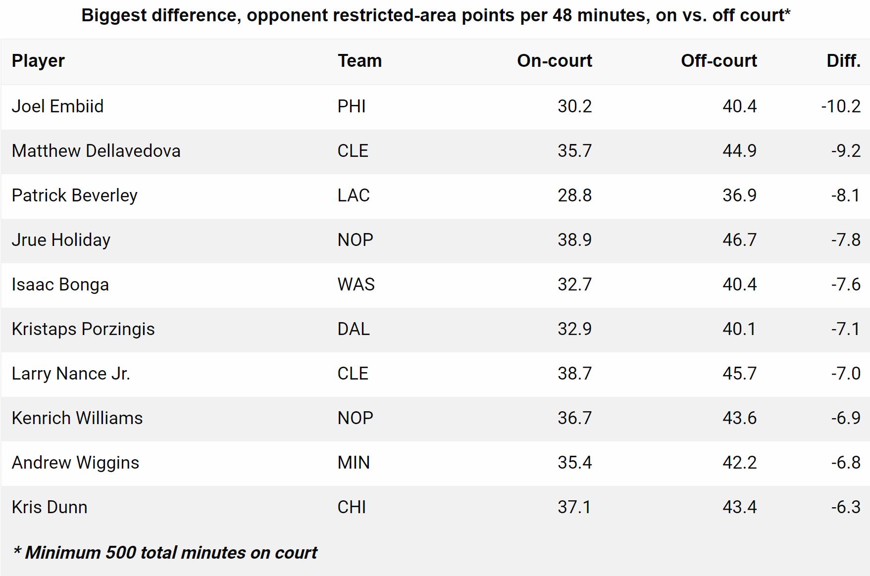
We’re going to use the same table we just used, shot_lineups, and filter it to keep only the made shots in the restricted area. Then we’ll create a column called slugOpp to tell us who was on the receiving end of the shot.
shots_players <- shots_lineups %>%
  filter(zoneBasic == "Restricted Area",
         typeEvent == "Made Shot") %>%
  mutate(slugOpp = ifelse(slugTeam == slugTeamHome, slugTeamAway, slugTeamHome)) %>%
  select(idGame, idEvent, slugTeam, slugOpp, lineupOpp)

shots_players
## # A tibble: 35,324 x 5
## idGame idEvent slugTeam slugOpp lineupOpp
## <dbl> <dbl> <chr> <chr> <chr>
## 1 21900014 11 ATL DET Andre Drummond, Bruce Brown, Markieff Morr~
## 2 21900014 18 ATL DET Andre Drummond, Bruce Brown, Markieff Morr~
## 3 21900014 40 ATL DET Andre Drummond, Bruce Brown, Markieff Morr~
## 4 21900014 71 ATL DET Andre Drummond, Bruce Brown, Markieff Morr~
## 5 21900014 96 ATL DET Andre Drummond, Bruce Brown, Derrick Rose,~
## 6 21900014 103 ATL DET Andre Drummond, Bruce Brown, Derrick Rose,~
## 7 21900014 125 ATL DET Derrick Rose, Langston Galloway, Luke Kenn~
## 8 21900014 176 ATL DET Langston Galloway, Luke Kennard, Markieff ~
## 9 21900014 181 ATL DET Langston Galloway, Luke Kennard, Markieff ~
## 10 21900014 219 ATL DET Andre Drummond, Bruce Brown, Markieff Morr~
## # ... with 35,314 more rowsWe know every player from the opposing lineup that was on the floor during the shot, but how about the players who were not? We’re going to add a column with every player who has played over the season per team, and then find the difference between the lineup on the court and these players (column not_in).
shots_players <- shots_players %>%
  left_join(lineup_stats %>%
              separate_rows(lineup, sep = ", ") %>%
              group_by(slugOpp = slugTeam) %>%
              summarise(every_player = paste(sort(unique(lineup)), collapse = ", "))) %>%
  mutate_at(vars(c(lineupOpp, every_player)), ~ str_split(., ", ")) %>%
  mutate(not_in = map2(lineupOpp, every_player, ~ setdiff(.y, .x)),
         not_in = map_chr(not_in, ~ paste(sort(.), collapse = ", ")),
         lineupOpp = map_chr(lineupOpp, ~ paste(sort(.), collapse = ", "))) %>%
  select(-c(every_player, slugTeam))

shots_players
## # A tibble: 35,324 x 5
## idGame idEvent slugOpp lineupOpp not_in
## <dbl> <dbl> <chr> <chr> <chr>
## 1 21900014 11 DET Andre Drummond, Bruce Brow~ Blake Griffin, Brandon ~
## 2 21900014 18 DET Andre Drummond, Bruce Brow~ Blake Griffin, Brandon ~
## 3 21900014 40 DET Andre Drummond, Bruce Brow~ Blake Griffin, Brandon ~
## 4 21900014 71 DET Andre Drummond, Bruce Brow~ Blake Griffin, Brandon ~
## 5 21900014 96 DET Andre Drummond, Bruce Brow~ Blake Griffin, Brandon ~
## 6 21900014 103 DET Andre Drummond, Bruce Brow~ Blake Griffin, Brandon ~
## 7 21900014 125 DET Derrick Rose, Langston Gal~ Andre Drummond, Blake G~
## 8 21900014 176 DET Langston Galloway, Luke Ke~ Andre Drummond, Blake G~
## 9 21900014 181 DET Langston Galloway, Luke Ke~ Andre Drummond, Blake G~
## 10 21900014 219 DET Andre Drummond, Bruce Brow~ Blake Griffin, Brandon ~
## # ... with 35,314 more rowsNow let’s turn each row into a player and his status (on or off the court) during every shot:
shots_individual <- shots_players %>%
  separate_rows(lineupOpp, sep = ", ") %>%
  separate_rows(not_in, sep = ", ") %>%
  pivot_longer(cols = c("lineupOpp", "not_in"),
               names_to = "inLineup",
               values_to = "namePlayer") %>%
  distinct(idGame, idEvent, slugOpp, inLineup, namePlayer)
We know every field goal in the restricted area results in 2 points, so we sum the total points for each player on and off the court.
shots_individual <- shots_individual %>%
  mutate(points = 2) %>%
  group_by(namePlayer, slugOpp, inLineup) %>%
  summarise(total = sum(points)) %>%
  ungroup()

shots_individual
## # A tibble: 1,134 x 4
## namePlayer slugOpp inLineup total
## <chr> <chr> <chr> <dbl>
## 1 Aaron Gordon ORL lineupOpp 1320
## 2 Aaron Gordon ORL not_in 810
## 3 Aaron Holiday IND lineupOpp 1010
## 4 Aaron Holiday IND not_in 1282
## 5 Abdel Nader OKC lineupOpp 550
## 6 Abdel Nader OKC not_in 1716
## 7 Adam Mokoka CHI lineupOpp 80
## 8 Adam Mokoka CHI not_in 2590
## 9 Admiral Schofield WAS lineupOpp 210
## 10 Admiral Schofield WAS not_in 2224
## # ... with 1,124 more rowsNow we need to find the number of minutes for each player’s status. The number of minutes on the court can be calculated from our lineup_stats table, but we still need the total while was off it. To find it, we’ll add the a column with the sum of minutes played by everyone on the team and divide it by 5 (number of players on the court at the same time). The difference from that total and the player minutes on the court will be the number of minutes off the court. Finally, we filter for the players that have played at least 500 minutes and find the value per 48 minutes.
shots_individual %>%
  left_join(lineup_stats %>%
              separate_rows(lineup, sep = ", ") %>%
              group_by(slugOpp = slugTeam, namePlayer = lineup) %>%
              summarise(totalTime = sum(totalTime)) %>%
              ungroup() %>%
              group_by(slugOpp) %>%
              mutate(totalTeam = sum(totalTime)) %>%
              ungroup() %>%
              mutate(totalTeam = totalTeam / 5)) %>%
  filter(totalTime >= 30000) %>%
  pivot_wider(names_from = inLineup,
              values_from = total) %>%
  mutate(timeOff = totalTeam - totalTime) %>%
  mutate(withPer48 = (lineupOpp * 2880) / totalTime,
         withoutPer48 = (not_in * 2880) / timeOff) %>%
  select(Player = namePlayer, Team = slugOpp, On_Court = withPer48, Off_Court = withoutPer48) %>%
  mutate(Difference = round(Off_Court - On_Court, 1)) %>%
  arrange(-Difference)
## # A tibble: 329 x 5
## Player Team On_Court Off_Court Difference
## <chr> <chr> <dbl> <dbl> <dbl>
## 1 Joel Embiid PHI 30.2 40.4 10.2
## 2 Matthew Dellavedova CLE 35.7 44.9 9.2
## 3 Patrick Beverley LAC 28.8 36.9 8.1
## 4 Jrue Holiday NOP 38.9 46.7 7.8
## 5 Isaac Bonga WAS 32.8 40.4 7.6
## 6 Kristaps Porzingis DAL 32.9 40.1 7.1
## 7 Larry Nance Jr. CLE 38.7 45.7 7
## 8 Kenrich Williams NOP 36.7 43.6 6.9
## 9 Andrew Wiggins MIN 35.4 42.2 6.8
## 10 Kris Dunn CHI 37.2 43.4 6.3
## # ... with 319 more rowsThis will be the last post on our series with play-by-play data, even though we are still going to use it in other posts. Thank you for reading!